Background Theory
Probability
Probability theory gives a mathematical context to understand how likely it is for events to occur. We encounter this on a daily basis. For instance, when driving to work, one might think of multiple routes and predict a “ballpark” estimate of how likely it is that one route will be faster than another. The weather is another great example of using probability to plan daily life. In the context of POD, probability is specifically giving us a measure of how likely an inspection is to detect a flaw (the event) of a given size.
It is important to remember, however, the context for why we are determining POD to begin with. An engineer is trying to determine the largest flaw that could be missed during ANY inspection performed in practice on an entire fleet. It is not enough to understand the uncertainty from one inspector, one serial number instrument, or one particular component under test. Life management and inspection intervals are based on the inspection being performed across the entire fleet, thus the uncertainty that needs to be considered for a POD study should account for the sources of variability across the entire fleet. Examples of parameters to vary over in a POD study include:
- Multiple serial number instruments and probes
- Multiple inspectors with varying experience and qualifications
- Multiple components with various geometric configurations
- Material variability
Random Variables and Distributions
An entire discussion of random variables and distributions would be well beyond the scope of this article. It is highly suggested that the reader unfamiliar with these concepts seek out more information from more comprehensive sources (for example, [6-8]). Here, these concepts will be introduced insofar as they contribute to the understanding of the concepts of how to develop a POD curve.
A random variable is a variable whose quantity cannot be known until performing an experiment. Furthermore, each time the experiment is performed, the value of the variable can change. In other words, a random variable is the numerical outcome of some random phenomenon. In the case of POD, a random variable is the outcome of an inspection. In fact, both signal values in â vs. a and hit/miss decisions are considered random variables.
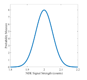
Random variables are defined by probability density functions (PDF) or probability mass function (PMF) in the case of discrete outcomes. These are functions that define a measure of the probability of a specific outcome of that variable. For instance, many readers will be familiar with a Gaussian (or normal) PDF, or the so-called bell curve with mean, and standard deviation, σ:

Figure 10. Gaussian probability density function describing the probability of specific signals strengths
The function that defines this curve is given by:

This equation is essentially describing the probability that, given a specific flaw of size a, the NDE sensor will record a specific signal strength, â.
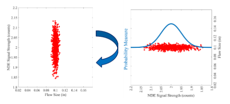
In practice, data is rarely perfectly Gaussian. In fact there are a great deal of distributions that can be used to describe data. However, to simulate the random signal strength in terms of a Gaussian random variable, if we were to record signals from a flaw of size 0.1”, we could plot the signal by putting a small amount of “jitter” on the x axis so that we can see all the data points. This can be seen in the left plot of Figure 11. What can be seen here is that there are more signals around the mean signal strength (in this case, μ=2) and the number of signals recorded at values further away from this value decreases. This can be described by the probability density in Fig. 10. If we rotate the left plot of Fig. 11 clockwise by 90 degrees, we can see how the probability density function describes the density of data as a function of signal strength. This will be important for understanding the transition from basic models to POD.

Figure 11. Image of signals plotted as a function of flaw size (jitter was added to the flaw size for visual representation) and the relationship between signal strength and the probability density function describing the signal.
Cummulative Distribution
One very important concept to understand the calculation of POD is the cumulative distribution function (CDF) of a random variable. The CDF(x) defines the probability that a random variable will have a value of x or lower. If the random variable is X, then the CDF is defined as:
CDF(x) = P(X≤x)
If the random variable, X, has a probability density function (PDF), f(x), then the CDF of X can also be written as:

In words, this basically says that the probability that the random variable, X, will have a value somewhere between -∞ and x is equal to the area under the curve of the PDF of the random variable from -∞ to x.
Why is this critical for understanding POD? It is important to remember the definition of detection for â vs. a inspections. In this scenario, we defined detection as a signal rising above a specific threshold. Detection means that â is greater than a specific number, âdec. Given that a is a random variable (by definition, the PDF of a integrates to 1), probability of detection can then be stated mathematically as:
POD(a) = P(â > âdec) = 1 - P(â ≤ âdec)
Thus, if we can predict the PDF of the signal at a specific flaw size, the POD(a) is the area under that PDF curve calculated from âdec to + ∞. Once we estimate β0 and β1 in equation (1), the PDF can then be directly taken from this equation and the distribution of ε.